

“Facts are stubborn things, but statistics are pliable.”
Mark Twain
DAX is the language native to Power BI and Analysis Services. It contains a large array of functions to accomplish many different things. From creating tables, columns, and measures, you cannot get very far in Power BI without getting into DAX at some point.
With the variety of functions available, some get used more than others. While I have no data on the subject, the lack of blogs and videos on DAX’s statistical functions does suggest that they are rarely used.
In this post, I plan to showcase various statistical functions. These functions are associated with normal, chi-squared, and Poisson distributions.
I will be using the Internet Sales fact table from the AdventureWorks sample data set provided by Microsoft for this post.
Sales Analytics: a Statistical DAX Function Use Case
Analyzing the Number of Orders per Customer
The first part of our analysis will be into the number of times a customer has made a purchase.
For a business, repeat customers are desirable. Below is a visual showing the number of customers by the number of purchases they have made.
In the data warehouse, the Internet Sales table covers the years 2011 to 2013. The visual separates the customers who made their first purchase in 2011 from those who first purchased in 2012 and 2013. For our purposes, we want to analyze customers from 2011. This allows time for additional orders in later years. It leads to a better long-term analysis.
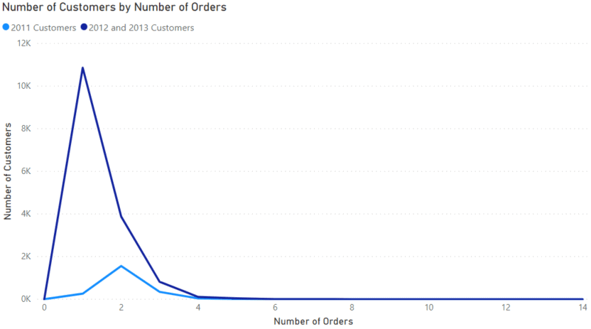
The basic DAX measure for this visual is below:
Normal and Chi-Squared distributions in Power BI
Now we can add some distributions and try to fit the 2011 customers. These distributions can then be used later to predict the number of repeat customers in the future.
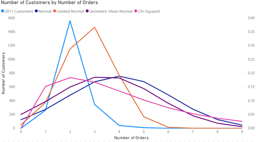
The first distribution we fit is the normal distribution using the NORM.DIST function in the expression below.
The function parameters include:
- the x-axis value
- mean from AVERAGEX
- standard deviation from STDEVX.P
- a choice for cumulative or not
The mean determines where the maximum of the distribution will be. The standard deviation determines how broad the distribution is. We are using the “.P” version of the standard deviation because these statistics are being calculated using the entire dataset.
If we only had a sample of the data, then we would have to use STDEVX.S.
The normal distribution here does not match the data all that great, so we can try some alternatives. The first two are variations of the normal distribution. The “Limited Normal” measure only used customers with 4 or less orders and fits better.
The “Geometric Mean Normal” measure replaces the AVERAGEX function with GEOMEANX. This is an alternative way to calculate an average by multiplying all the values together and taking the n’th root.
This method gives a value better representing datasets with large outliers that could dominate the data set.
The last distribution is the Chi-Squared distribution using the CHISQ.DIST function.
This function takes the value of the x-axis and a parameter called degrees of freedom. I found that putting the average in did a good job of approximating the curve. The advantage of the Chi-Squared distribution in this example is that it is zero at zero, like our data.
Super Customers
Let’s say we classify customers who have made more than five purchases as Super Customers. These are customers we deem likely to purchase regularly over time. Also, we would like to offer them special promotional offers to ensure their loyalty. We want to estimate, what percentage of our customers are Super Customers over time.
For this, we need to change our distributions to use TRUE() in the last argument which changes the functions to cumulative ones. Below are the cumulative distributions. It uses:
- the Limited Normal distribution (parameterized only using customers with 4 or fewer orders)
- the Chi-Squared distribution
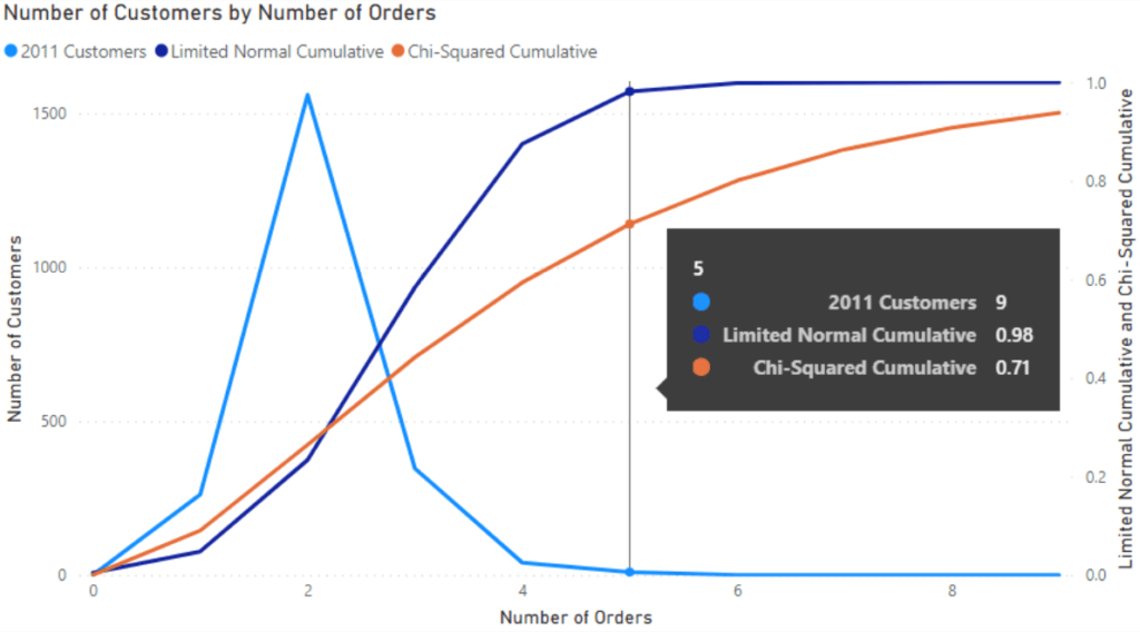
Moving left to right then gives us a running total of the distribution. Hovering over 5 orders brings up the tooltip showing the fractions of each distribution, 0.98 for the Normal one and 0.71 for the Chi-Squared.
The Limited Normal Distribution fits the data well. As a result, we can likely conclude the following: 2% of customers will become super customers within a three-year period.
Analyzing the Number of Orders per Day
Sales from an online store need to be fulfilled by employees in the shipping centre. A single employee can only handle a certain number of packages per shift. Let’s just say that it’s 20 for this example. We need to ensure that enough people are working to cover all the orders coming in.
Poisson Distribution in Power BI
The Poisson distribution estimates the number of events in each duration. For example, website orders are not correlated, as one sale doesn’t affect the next. But, there is an average over time.
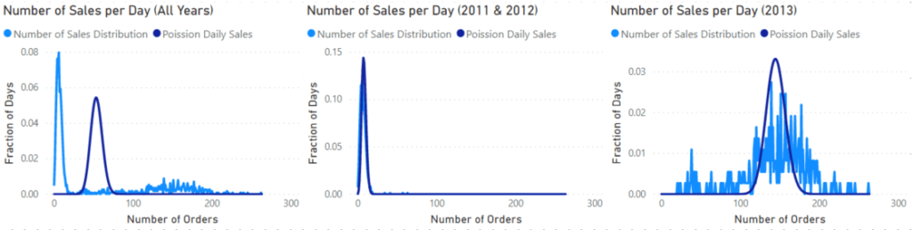
The visuals above show the number of orders by the number of days with those orders. The first visual on the left shows the whole data set which shows two peaks. A bit of digging shows that the sharp peak on the low end of the orders came from 2011 and 2012, while the broader peak came from 2013. These years are split out in the middle and right visual.
In all these visuals, the dark blue line shows the Poisson distribution for the data using the POISSON.DIST function.
The POISSON.DIST function takes three arguments. The first is the x-axis value, then the average of the data set and a Boolean value determining if the function is cumulative or not.
Using the 2013 data, let’s investigate the problem of making sure we have enough workers filling orders. On the 2013 visual, we can add a new measure using the previous Poisson distribution, but changing it to be cumulative.
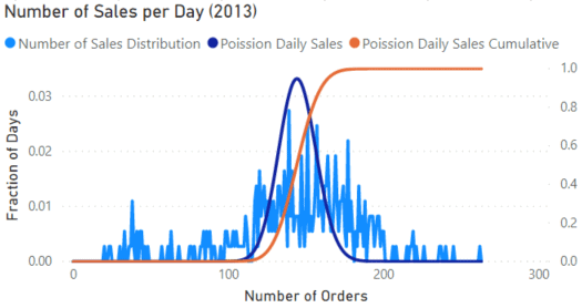
Then we must hover over the visual until we find the point where the value of the ‘Poisson Daily Sales Cumulative’ measure is 0.95. This shows that 95% of the days are below that number of orders. The value comes to 164 orders per day.
According to the distribution then, if we had 164/20 = 9 (rounding up) employees in the warehouse, we should be fine filling orders at least 95% of the time.
Conclusion
In this blog post, I’ve introduced and used several of DAX’s statistical functions to explore the data in the AdventureWorks Data Warehouse. DAX contains many more of these functions for many purposes. This post was just a taste of what is possible, and I encourage you to explore DAX’s statistical functions on your own.
What is a DAX function?
A DAX function is a set function used in an expression to perform actions based on specified inputs. There are many types of DAX functions. Learn more from Microsoft documentation of DAX here.
Don’t miss out on the latest updates and tips about DAX and Power BI from our experts at Iteration Insights! To stay informed and enhance your skills, make sure to follow our content. Let Iteration Insights empower you with the knowledge to excel in your data-driven journey.