
Power Query is a powerful tool available in both Excel and PowerBI that can be used to transform, manipulate, and cleanse data. Amongst the plethora of functions utilized in Power Query, a commonly used transformation is Merge Queries.
This is used when a user wants to combine two tables, and with Merge Queries, you are provided multiple ways to suit your needs. Understanding the differences between the different join types available is a foundational skill in data analytics.
Sections
Sample Data
Before getting any further, here are the sample tables we will be using to showcase the features of Merge Queries.
Sales
| EmployeeID | CountryID | SaleAmount |
| 1 | 1 | 100 |
| 2 | 2 | 250 |
| 1 | 5 | 100 |
| 6 | 1 | 300 |
| 3 | 5 | 1000 |
| 7 | 4 | 450 |
| 4 | 3 | 500 |
| 2 | 1 | 650 |
| 3 | 4 | 900 |
| 2 | 3 | 800 |
DimSalesperson
| EmployeeID | Name |
| 1 | Isaac Clarke |
| 2 | Jesse Faden |
| 3 | Joel Miller |
| 4 | David Martinez |
| 5 | Faith Conners |
DimCountry
| CountryID | Country |
| 1 | Canada |
| 2 | Japan |
| 3 | India |
| 4 | Australia |
| 6 | Italy |
Note that the Sales table contains ID columns that can be matched to the ID columns in the dimension tables. Establishing this relationship is necessary for the Merge Queries function to work.
Merge Queries Selection
First, in Power Query, you must select the base table you wish another table to join on to from the Queries pane. Then, Merge Queries can be selected from the Home tab under the Combine category.
Clicking the drop-down arrow shows you two options for how Merge Queries will provide your result. The first option “Merge Queries” will apply the transformation to the selected table. The second option, “Merge Queries as New” will result in a new table being created with the merge performed.

After selecting the option you require, the following window will appear.
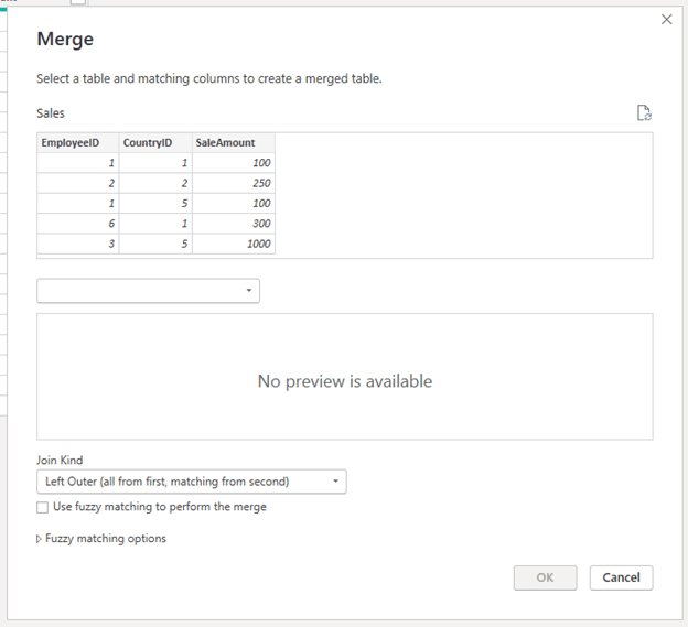
A preview of the table you selected will be shown at the top. This is your LEFT table. Then, from the drop-down, you will select the second table that you wish to join to the first (we will select DimCustomers). A preview of the said table will then appear. This is your RIGHT table.
The next step is to select the key columns in each table that correspond to one another to establish a relationship on which the merge can be performed on. In this case, the match will occur on EmployeeID.
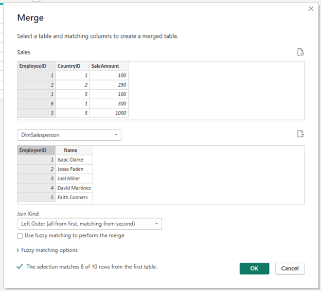
Power Query tells you how many matches you have between the selected columns on the bottom depending on the Join Kind you have selected.
Join Types
Now we will go into the different types of join functions Power Query has made available to us.
Left Outer (all from first, matching from second)
The most common join type when performing data manipulation. With your first table being your left table, and your second being your right, this join takes all the rows from the left table and attempts to match it with the corresponding values from the right. Let’s go ahead and click “OK” to perform this type of join.
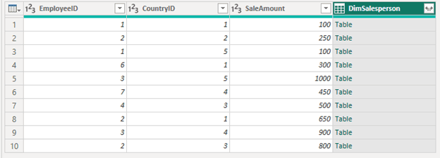
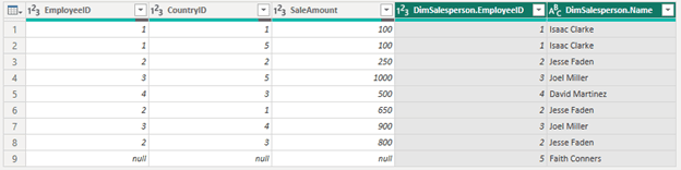
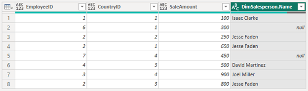
As expected, we still have all 10 rows of data from our first (left) table. Now let’s expand the DimSalesperson data to see how it was merged.
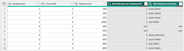
We can see that there are null values in some rows, 2 to be exact, just as Power Query told us there would be (8 of 10 rows would match, leaving 2 unmatched). This is because the Sales table has EmployeeID numbers that are not found in the DimSalesperson table (EmployeeIDs 6 and 7). With no match to be found, only null values can be returned.
Right Outer (all from second, matching from first)
This type of join works in the opposite direction compared to a left join. With this join, all rows of the right table will be included, and only the rows that have a match from the left table. When selecting this option in our example, Power Query tells us 4 of 5 rows will match, which is reflected in the result.
9 rows have been returned. 8 rows from the left table matched to the right table (rows with EmployeeIDs 6 and 7 have been removed), and an additional row has been returned from the right table. This row corresponds to EmployeeID 5, which exists in the DimSalesperson table, but not the Sales table. With no match to this row in the left table, the values returned in the columns of the Sales table are null.
Full Outer (all rows from both)
Combining both of these joins together reflects a full outer join. This will return all rows from both tables, whether or not they match.

As expected, we have 11 rows returned, which coincides to the results of a left and right join.
Inner (only matching rows)
If you want your results to return only the values that match in both tables, you would use an Inner join. Inner joins acts somewhat as a “filter” if you want to remove any data that could return a null value through other join types, as shown below.
Rows corresponding to EmployeeIDs 6 and 7 have been removed, and only the matching rows remain. EmployeeID 5 from the DimSalesperson table also isn’t here as it does not have a match to the Sales table. As a result, no null values are seen.
Left Anti (rows only in first)
Now we have our anti joins. As you might suspect, they are the inverse of the normal Left and Right Outer joins. With a Left Anti join, the rows returned are those in the left table that do not have a match in the right table. Selecting this match in the Merge Queries window, Power Query will tell you “The selection excludes 8 of 10 rows from the first table”.

As noted, only two rows remain with EmployeeIDs 6 and 7, that do not have a match to the DimSalesperson.
Right Anti (rows only in second)
Finally we have our Right Anti join. As with the Left Anti join, this will exclude all rows that have a match, but in the right table instead. Can you guess how many rows will remain based on our examples?

If your answer was 1, you were correct! EmployeeID 5 only exists in the DimSalesperson table, and does not have a match to the Sales table, leaving it the only row returned.
Putting It Together
Now knowing what these joins do, in some cases you may want to perform more than one kind of join on a table depending on your use case. Let’s look at an example using our sample data.
Say you have been tasked with creating a table that lists all sales in the countries populated in the database. We also want to see the names of the Salespeople who performed the sale, including those that are missing from the database. How would you achieve this?
First, we need to determine what makes sense to be your first (left) table. As we want to determine sales, logically our starting point will be the Sales table. This will be our left table.
Now let’s perform the first operation to include only the sales that occurred in countries from the DimCountry table, in this case CountryIDs 1, 2, 3, 4, and 6. The Sales table has CountryID 5 listed, which does not appear in the DimCountry table, and as such we want these rows removed.
We could potentially use the right join to achieve this. Let’s see what happens.
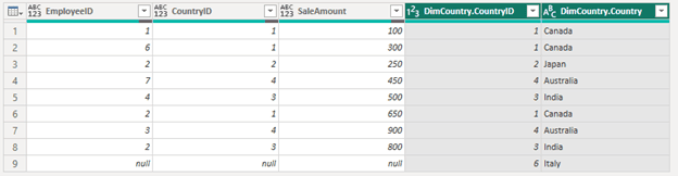
As desired, rows with CountryID 5 have been removed, but unfortunately, we are returned a row with null values. This means there is no match to CountryID 6 (Italy) from the DimCountry table in the Sales table. For our purposes, the resulting table should not include any rows where sales did not occur, so a different join option should be used.
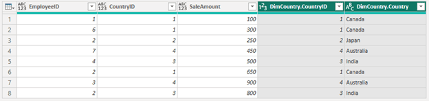
A better option is an inner join. Selecting this returns what we require, only sales from Canada, Japan, India, and Australia, and no rows corresponding to Italy. The expanded columns can be removed leaving only the data from the Sales table. We will now refer to this table as Sales2.
Now moving on to the next part, we want to see the names of the salespeople who performed these sales, including those whose names are not in the database.
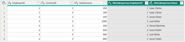
Again, it makes sense for our left table to be the Sales2 table, and our right will be DimSalesperson. Since we now want to keep all the sales, as in all the rows in the Sales2 table, a left join makes sense. Selecting the join and expanding the Name column results in the following.
We have the matching names from the DimSalesperson table, as well as the indication that EmployeeID 6 and 7 do not correspond to a name in the database. We are now done!
Conclusion
Joins are powerful functions used in data analytics every day. The concept behind the different join types in Power Query are similar to SQL based join functions and are incredibly powerful tools. Understanding the differences opens many possibilities for manipulating tables to suit your needs.
