
Section
View the tutorial in the Power BI Dashboard or keep scrolling for text!
Wait… What is Linear Regression?
Linear Regression is a statistical model applied to businesses to help forecast events based on historical trend analysis. Simple Linear regression uses one variable, called the independent variable. The independent variable predicts the outcome of another variable called the dependent variable.
A Linear Regression Model is created by fitting a trend line to a dataset where a linear relationship already exists.
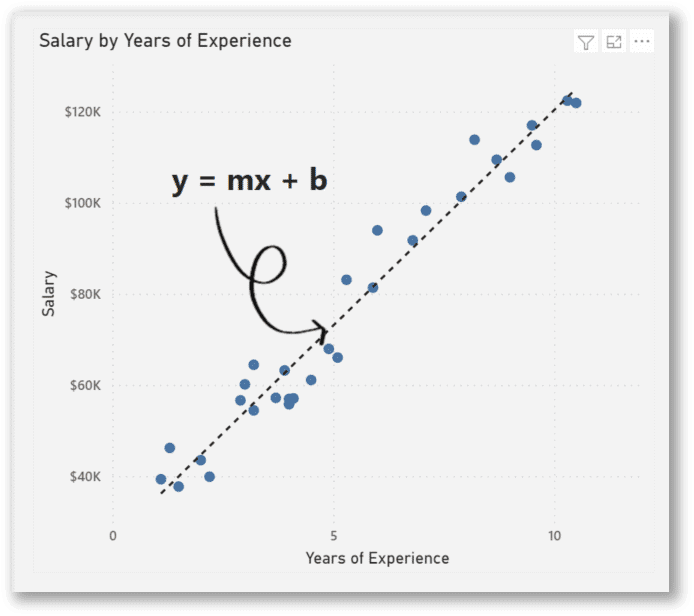
This trend line has the equation of y = mx + b and is used to make estimates.
(Note: To successfully implement Linear Regression on a dataset, you must follow the four assumptions of simple Linear Regression. Statistical tests can be performed to check the validity of the model, however, this process is beyond the scope of this tutorial.)
Tutorial
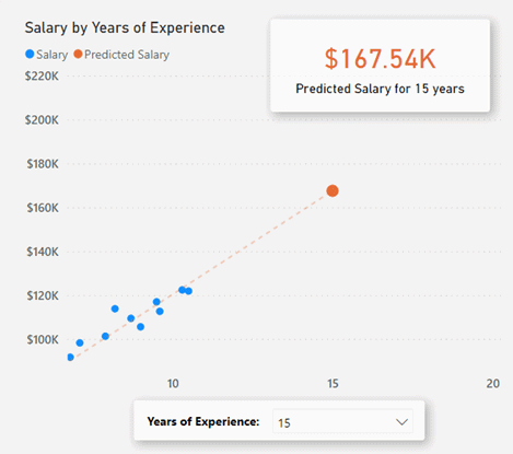
Consider this Scatterplot visual. Illustrated is the relationship between Years of Experience and Salary at a fictional company. By fitting a trend line to the Scatterplot, we can see that the more years of experience an employee has, the more they will get paid. Our y data points represent Salary in thousands, and the x data points represent Years of Experience.
Click Here to Follow the Tutorial in Power BI
According to the data above, if an employee has 15 years of experience, how much will they be paid? What about 20 years of experience? 30 years?!
Let’s try this out!
Steps we need to take:
- Create calculated columns and measures for the components of the equation of a line
- Create a What-if parameter for the x-values
- Create the measure of the equation of a line and insert a card visual with the measure
If you would like to follow along, this tutorial is demonstrated using the Salary_data dataset from Kaggle.com.
Step 1: Create Calculated Columns and Measures
The formula for the equation of a line is y = mx + b.
Where:
y = How far up the y axis
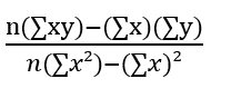
m = Slope (Change in y divided by change in x) =
x = How far along the x axis
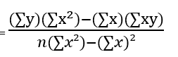
b = b-intercept (The value of y when x = 0) =
After finding out m and b with some calculations, we can input any data point for x and the output will be y.
We are going to create this formula using DAX calculated columns and measures.
These are the Calculated Columns we need to make and their DAX syntax:
| Math Formula | DAX Formula |
| x² | xsq = Salary_Data[Years of Experience]^2 |
| xy | xy = Salary_Data[Years of Experience]*Salary_Data[Salary] |
These are the Measures we need to make and their DAX syntax:
| Math Formula | DAX Formula |
| n | n = COUNTROWS(Salary_Data) |
| ∑xy | xysum = SUM(Salary_Data[xy]) |
| ∑x | xsum = SUM(Salary_Data[Years of Experience]) |
| ∑y | ysum = SUM(Salary_Data[Salary]) |
| ∑x² | xsqrsum = SUM(Salary_Data[xsq]) |
| (n(∑xy)-(∑x)(∑y))/(n(∑x²)-(∑x)²) | m (Slope) = DIVIDE( [n]*[xysum]-[Xsum]*[Ysum], [n]*[xsqrsum]-[Xsum]^2, 0 ) |
| ((∑y)(∑x^2)-(∑x)(∑xy))/(n(∑x²)-(∑x)²) | b (Intercept) = DIVIDE( [ysum]*[xsqrsum]-[Xsum]*[xysum], [n]*[xsqrsum]-[Xsum]^2, 0 ) |
Step 2: Setting up a What-if parameter
Now that we have performed our calculations, for any number we insert into x, the formula will predict y.
To demonstrate this, we will be using a What-if parameter with a slicer.
A What-if parameter allows you to create an interactive slicer with a variable to visualize and quantify another value in your report.
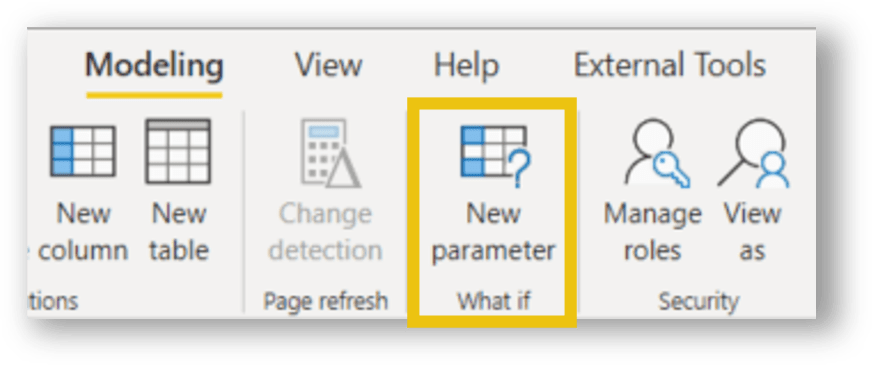
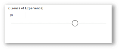
After clicking the What-if parameter on the modeling ribbon, we can input these values:
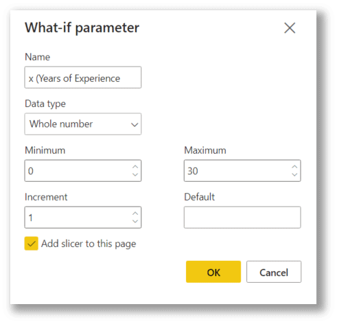
Name: x (Years of Experience)
Data type: Whole Number
Minimum: 0
Maximum: 30
Increment: 1
Add slicer to this page: Yes
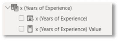
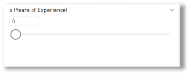
Once we press ‘OK’, the What-if parameter will have generated a series of x values and a slicer to use for our What-if scenarios.
Step 3: Complete the measure for the equation of a line and visualize
Finally, we create the Predicted Salary measure that contains the complete formula for the regression equation of a line y = mx + b, using the components we have created previously.
| Math Formula | DAX Formula |
| y = mx + b | Predicted Salary = ([m (Slope)]* ‘x (Years of Experience)'[x (Years of Experience)Value]+ [b (Intercept)] ) |
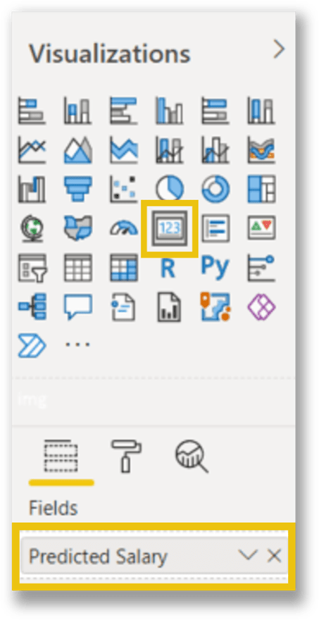
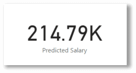
We can now insert a card visual in the report and select the measure Predicted Salary for the field.
We can test the calculation by toggling the slicer left and right. This action will interact with the Card visual and represent the predicted salary for the selected Years of Experience.
Create awesome visualizations!
There are many ways to visualize the prediction that we have set up using Linear Regression. A toggle and a card provide enough information, but we can also integrate that calculation into a chart to visualize the existing data and the predicted value.
Now you now have the power to make predictions!
Conclusion
Linear Regression helps forecast future events by fitting a trend line to the model and using the equation of a line to predict our values. By following the steps in this tutorial, you can implement Linear Regression on a valid dataset and make estimations on future values. Try this tutorial out with a public dataset and share your findings!
Resources
If you would like to learn more statistical functions in DAX, check out Stephen Zielke’s blog post!
This tutorial was in reference to this YouTube video: DAX Fridays! #135: Linear Regression in Power BI.
The dataset used for this tutorial is called Salary_Data found a Kaggle.com.
The formulas used for Linear regression were referenced from Linear Regression: Simple Steps, Video. Find Equation, Coefficient, Slope – Statistics How To.
